
Every quick-service operator has a drive-thru timer, and every one of them can tell you their average service time to the second. Far fewer can tell you which stage of the lane produced that number, and that gap is where most improvement efforts stall.
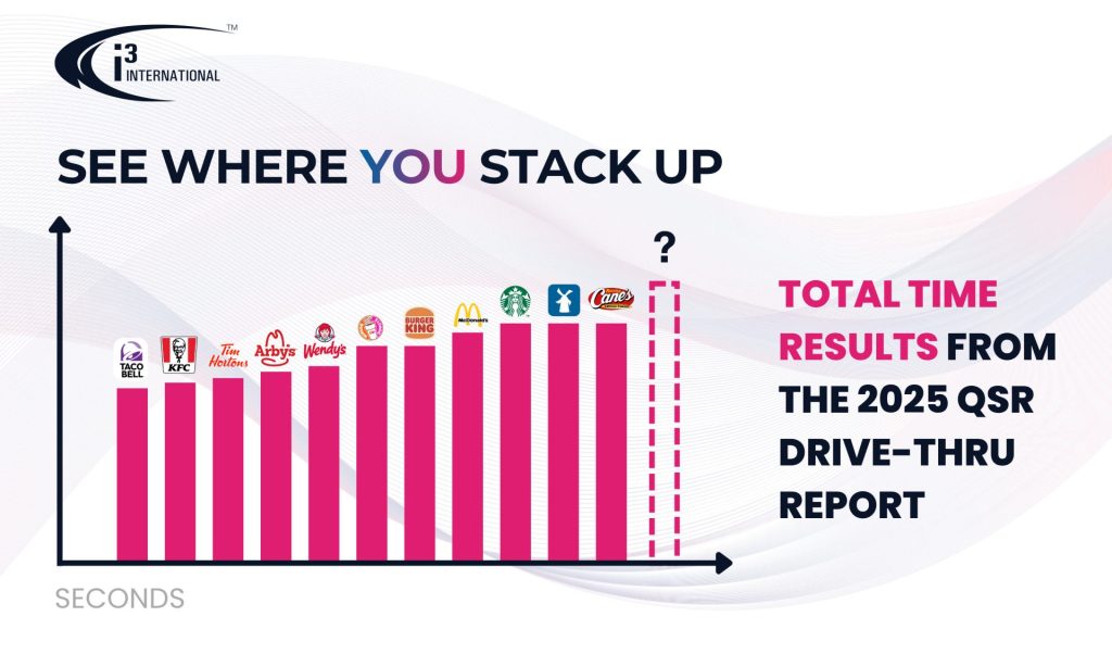
The industry-wide picture sets the scale. The 2025 QSR Drive-Thru Report, run by Intouch Insight across 13 U.S. chains with 165 mystery shops per brand, put average total service time at 4 minutes 15 seconds, ten seconds slower than 2024. Order accuracy fell to 87%, down from 89% the year before.
This guide covers how to run a proper bottleneck analysis across a multi-location estate: how to segment total service time into stages, how to identify the actual constraint, how to separate problems that need capital from problems that need scheduling, and how to compare locations without letting the average hide your worst performers.
Not sure how your restaurant is performing? Use the Drive-Thru Performance Calculator to benchmark against recent industry leaders.
Why Total Service Time Is the Wrong Diagnostic
Total drive-thru time is an outcome. It tells you the system is slow. It does not tell you which part of the system is slow, and without that, every remedy is a guess.
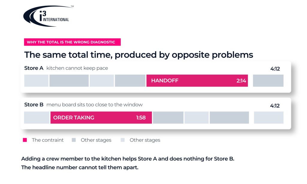
Consider two locations reporting an identical total. At the first, orders are taken quickly but the kitchen cannot keep pace, so cars stack at the presentation window while food is assembled. At the second, the kitchen is comfortably ahead but the menu board is positioned badly, so order-taking runs long and everything downstream inherits the delay.
Same number. Opposite problems. Opposite fixes. Adding a crew member to the kitchen helps the first location and does nothing for the second.
This is why estates that chase the headline number tend to plateau. They apply the same intervention everywhere, it works in some locations and not others, and the average barely moves.
The same study makes the point with hard numbers. Accurate orders moved through the drive-thru 49 seconds faster than inaccurate ones. Accuracy is not a service-quality metric that happens to sit alongside speed; on that evidence it is one of the largest single determinants of speed. An operator watching only total time would never see it, because the cause and the symptom are recorded as separate things.
The Drive-Thru as a Serial Queue
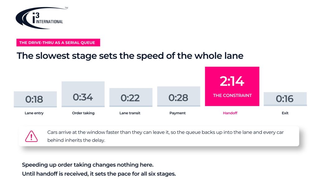
A drive-thru is a sequence of stages, and each car passes through them in order. Total time is the sum of the time spent in each stage plus the time spent waiting between them.
The stages that matter for analysis:
1- Lane entry and queue formation. From the moment a vehicle enters the property to the moment it reaches the ordering position.
2- Order taking. From arrival at the menu board to order confirmation.
3- Lane transit. Movement from the ordering position to the payment window, including any pull-forward.
4- Payment. Card, cash, or mobile, including any transaction that needs correcting.
5- Handoff. From payment completion to the food leaving the window.
6- Exit. Clearing the lane so the next vehicle can advance.
The critical property of a serial queue is that the slowest stage sets the throughput of the entire system. This is the constraint principle from Eliyahu Goldratt’s Theory of Constraints, set out in The Goal (1984) and applied in manufacturing and logistics for four decades. A drive-thru is a textbook case of it, and the principle is underused in restaurant operations mainly because the reporting stops at the total. If handoff can process one car every 90 seconds, it does not matter how fast order-taking runs. Cars will arrive at the window faster than they can leave it, the queue will back up into the lane, and the total time for every subsequent car will grow.
That slowest stage is your constraint. Everything else is noise until it is fixed.
Where Time Actually Goes: Four Areas to Analyze
1- Order Taking
Order taking is the first place delay compounds, because every second lost here is inherited by every stage downstream and by every car behind.
What to measure: time from vehicle arrival at the board to order confirmation, split by daypart. Track order modification rate and repeat-back frequency separately, since both signal a communication problem rather than a speed problem.
What the evidence shows: the 2025 study isolates several order-taking factors and quantifies each against accuracy, which in turn drives the 49-second gap above.
| Factor | Effect on order accuracy |
|---|---|
| Order confirmation board displaying correctly | +26 points (accuracy fell to 64% when incorrect) |
| Speaker interaction clear and understandable | +16 points |
| Speaker volume loud enough to hear the employee | +11 points |
| Customer did not have to repeat the order | +12 points |
Three of those four are equipment and installation problems rather than staffing or training problems, which is not where most operators look first.
What good analysis looks like: compare order-taking duration against order complexity. If long orders and short orders take similar time, the constraint is the interaction rather than the order itself, which points at audio hardware or the confirmation board. If duration scales with complexity, the constraint is the menu or the POS flow.
2- Lane Flow
Lane flow covers everything about how vehicles physically move through the space. It is easily mistaken for a staffing problem, because a queue caused by geometry and a queue caused by understaffing look identical in the total.
What to measure: transit time between stages, queue depth at each position, and how often vehicles are held at a position with nothing in front of them.
Common causes: lane geometry that prevents cars from advancing independently, single-lane configurations where one slow order blocks everyone, pull-forward practices that clear the window but move the delay rather than removing it, and merge points that stall entry.
What good analysis looks like: a car held at a position with clear road ahead means the stage in front is the constraint. A car moving freely into a queue means the constraint is further down. Mapping where vehicles stop, rather than how long they take overall, locates the bottleneck faster than any other single measurement.
On pull-forward: moving a car to a waiting bay improves the timer reading and does not improve the customer’s wait. If pull-forward rate is climbing while total time is flat, the estate is managing the metric rather than the operation. Track it as its own number.
3- Handoff
Handoff is where kitchen throughput and lane throughput meet. Two independent capacity limits collide at one window, and whichever is lower governs it.
What to measure: time from payment completion to bag out the window, and the proportion of cars waiting at the window for food rather than for a transaction.
Common causes: kitchen production not sequenced against lane order, assembly staged too far from the window (motion waste, in Lean terms), items with long cook times not started at order entry, packaging and drinks handled serially where they could run in parallel, and equipment faults that surface as small repeated delays.
What good analysis looks like: separate transaction time from food-wait time. These are two different failures with two different owners. A window that is fast at transactions and slow at food has a kitchen sequencing problem. A window slow at both has a staffing or process problem at the window itself.
4-Staffing
Staffing sits across all four stages rather than inside any one of them, which is exactly why it gets blamed for problems it did not cause and credited for fixes it did not deliver.
What to measure: stage-level timings mapped against actual staffing levels and shift boundaries, not scheduled levels. Track performance across shift changes specifically.
Common causes: headcount planned against average demand rather than peak, which is the classic capacity-planning error in any queueing system, breaks scheduled into rush periods, shift handovers that pause the line, and roles doubled up so one person is the constraint on two stages at once.
What good analysis looks like: overlay timing data on the actual roster. If a stage degrades at consistent times that align with breaks or handovers, the fix is scheduling. If a stage is slow regardless of who is working or how many, the fix is process or equipment, and adding people will not help.
How to Run the Analysis: A Five-Step Framework 
Step 1: Segment the total
Break total service time into the stages above. Any analysis that starts and ends with the headline number cannot identify a constraint. This step is the whole foundation, and it is the one most estates skip.
Step 2: Find the constraint
Identify the stage with the lowest throughput, not the longest duration. These are different things. A stage can take a long time and still not be the constraint if it processes cars in parallel. Look for where vehicles queue, because a queue always forms immediately in front of the constraint.
Step 3: Separate chronic from episodic
Chronic bottlenecks are present in every shift regardless of conditions. Lane geometry, menu board position, equipment capability, and kitchen layout are chronic. They need capital or physical change, and no amount of scheduling fixes them.
Episodic bottlenecks appear under specific conditions: a daypart, a staffing level, a particular crew, a weather pattern. They need process, training, or scheduling changes.
Confusing the two wastes budget in both directions. Chronic problems get met with more labour that cannot fix them, and episodic problems get met with capital that was never needed.
Step 4: Compare across locations, not against the average
An estate average is the least useful number in a multi-location analysis, because it hides exactly the locations you need to find. A district averaging a healthy figure can contain two locations performing far worse, and those two are where the recoverable time actually sits.
Rank locations by stage rather than by total. This surfaces patterns that totals conceal: a group of locations with the same handoff problem, or one location whose order-taking is dragging an otherwise strong district.
Step 5: Fix one constraint, then re-measure
When the constraint is relieved, the constraint moves. The stage that was second-slowest is now setting throughput. This is expected and it is the point. Improvement in a serial system is a sequence of constraints, addressed one at a time, with measurement between each.
Changing several things at once means you learn nothing about which one worked.
What This Requires From Your Systems
Stage-level analysis needs data most drive-thru timers do not produce on their own. A timer that reports total time and nothing else cannot support any step above Step 1.
The capability set that makes this analysis possible:
- Stage-level timing tied to individual vehicles, so total time can be decomposed rather than estimated.
- Video linked to timing data, so an anomalous stage duration can be reviewed rather than guessed at. A 90-second handoff means nothing until someone sees what happened during it.
- Transaction data joined to both, so voids, corrections, and payment failures show up as the timing events they are.
- Cross-location reporting in one place, so stage-level comparison across an estate is a report rather than a project.
i3 delivers that set as one platform. Stage-level timing tied to each vehicle, with the POS record and the footage attached (Velocity Drive-Thru Timer), produces the segmented measurement Step 1 depends on. Service-speed analytics (i3Ai Speed-of-Service) apply that measurement across every location, which turns Step 4’s stage-level ranking into a report rather than a project. Exception-based transaction reporting (Smart-ER) links voids and corrections to their footage, and that matters at the payment stage, where a correction and a delay are the same event. Live queue alerting (i3Ai Q-Alert) surfaces buildup while it is still happening rather than in a report the following week. People counting (i3Ai People Counting) and heat mapping add the volume and movement context behind the numbers, and a cloud-managed platform (i3 CMS) holds the whole estate in one view.
i3’s Velocity Drive-Thru Timer brings POS, video, and timing together so stage durations sit alongside the footage and the transaction that produced them. i3Ai Speed-of-Service technology applies that measurement across locations, and i3’s Ai Q-Alert surfaces queue buildup while it is still happening rather than in a report the following week. Smart-ER links transaction exceptions to video, which matters at the payment stage where a correction and a delay are usually the same event. Trajectory Analysis and i3Ai People Counting add the movement and volume context behind the numbers, and CMS puts the whole estate in one view.
The point of the platform is not more numbers. It is that the numbers arrive already attached to the reason.
How Do I Reduce Drive-Thru Service Times Across My Restaurants?
To answer directly: reducing drive-thru service times across multiple locations requires four things in sequence.
1- Segment total service time into stages at every location. Order taking, lane transit, payment, and handoff each need their own measurement, because total time cannot identify a constraint.
2- Find the constraint at each location individually. The slowest stage sets throughput for the whole lane, and it differs between locations that report identical totals.
3- Separate chronic bottlenecks from episodic ones. Chronic problems are physical and need capital. Episodic problems are conditional and need scheduling or process change. Applying the wrong remedy wastes both budgets.
4- Compare locations by stage rather than by average, then fix one constraint at a time and re-measure. When a constraint is relieved it moves, and the next one becomes visible only after the first is addressed.
The estates that improve fastest are the ones that stopped treating the drive-thru as a single number and started treating it as a sequence of measurable stages.
Frequently Asked Questions
What is drive-thru bottleneck analysis?
Drive-thru bottleneck analysis is the practice of breaking total service time into individual stages, such as order taking, lane transit, payment, and handoff, then identifying which stage has the lowest throughput. That stage is the constraint, and it sets the speed of the entire lane regardless of how fast the other stages run. The analysis locates the constraint so improvement effort goes to the stage that is actually limiting service rather than the one that appears slowest.
Why is my drive-thru slow even though we are fully staffed?
Full staffing does not resolve a constraint that is physical or procedural. If the bottleneck is lane geometry, menu board position, kitchen sequencing, or equipment capability, adding people cannot relieve it, because the limit is not labour. Stage-level measurement distinguishes the two: a stage that runs slow regardless of staffing level indicates a chronic constraint needing process or capital change, while a stage that degrades only at certain times indicates an episodic constraint that scheduling can address.
What is the difference between a chronic and an episodic drive-thru bottleneck?
A chronic bottleneck is present in every shift regardless of conditions, and typically comes from physical layout, equipment, or sequencing. It requires capital or structural change. An episodic bottleneck appears only under specific conditions such as a daypart, a staffing level, or a shift handover, and responds to scheduling, training, or process change. Treating one as the other wastes budget in both directions, which is why the distinction is worth making before any money is committed.
Does pull-forward actually reduce drive-thru times?
Pull-forward improves the timer reading and does not reduce the customer’s total wait, because the delay is relocated rather than removed. It has legitimate operational uses, particularly in keeping a lane clear for orders that are ready. Tracking pull-forward rate as its own metric alongside total service time prevents a rising pull-forward rate from being read as an improvement in speed.
How should multi-location operators compare drive-thru performance between restaurants?
Rank locations by stage rather than by total service time. An estate or district average conceals the outliers that hold the most recoverable time, and two locations reporting identical totals frequently have entirely different constraints. Stage-level ranking also surfaces patterns across the estate, such as a cluster of locations sharing the same handoff problem, which points to a systemic fix rather than site-by-site remediation.
What data do I need to run this analysis?
Stage-level timings tied to individual vehicles, video linked to those timings so an unusual duration can be reviewed rather than assumed, transaction data joined to both so payment corrections appear as the timing events they are, and cross-location reporting in a single view. A timer reporting only total service time supports none of the analysis beyond the first step.
Ready to Find Your Constraint?
Book a demo with i3 to see how multi-location QSR operators measure drive-thru performance stage by stage, across every restaurant, in one platform.